8.1: The Binomial Distribution
The binomial distribution is frequently useful in situations where there are two outcomes of interest, such as success or failure. It is often used to model real-life situations, and it finds its way into many extremely useful and important statistical applications and computations.
The Binomial Setting:
(1) Each observation is in one of two categories: success or failure.
(2) A fixed number, n, of observations.
(3) Observations are independent .
(4) The probability of success is the same for each observation.
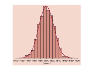
If a count, X, has a binomial distribution with number of observations, n, and probability of success, p, then
Mean(X) =
Standard Deviation(X) =
The probability that one will get exactly k successes is
On the TI-83, binompdf(n,p,k)
The probability that the sample contains k or fewer successes is binomcdf( n,p,k)
The Binomial Setting:
(1) Each observation is in one of two categories: success or failure.
(2) A fixed number, n, of observations.
(3) Observations are independent .
(4) The probability of success is the same for each observation.
If a count, X, has a binomial distribution with number of observations, n, and probability of success, p, then
Mean(X) =
Standard Deviation(X) =
The probability that one will get exactly k successes is
On the TI-83, binompdf(n,p,k)
The probability that the sample contains k or fewer successes is binomcdf( n,p,k)
8.2: The Geometric Distribution
The Advanced Placement Statistics Syllabus states that students need only know how to obtain geometric probabilities through simulation. The geometric setting is somewhat similar to the binomial setting, the basic difference being that the geometric setting does not have a fixed number of observations.
The Geometric Setting:
(1) Each observation is in one of two categories: success or failure.
(2) The probability of success is the same for each observation.
(3) Observations are independent.
(4) The variable of interest in the number of trials required to obtain the first success.